What is a Spin Glass?
In an attempt to motivate myself into keeping this updated, I’ll try to write a few notes on what spin glasses are and why we care. Our first example will be glass (mostly SiO2), the following is a snapshot of its atomic structure.
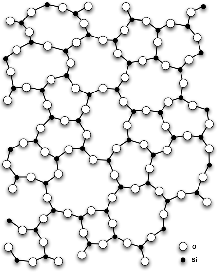
As you can see the structure is irregular and looks slightly random. Why is this the case? It’s because not all atoms are happy with their magnetic spin alignment! The atoms are forced into a frustrated position from the other atoms in the system (I’m vague on “other “atoms because this is one of our key choices in the working model). It may be better to call these objects frustrated magnets, since that’s what they are, though the name spin glass comes from trying to understand the structure of atoms with spins frozen in place (like glass!)
To begin our study, we need a basis for the model of the interaction of these atoms. The most famous to date(that I know of) is the Sherrington-Kirckpatrick Model. The model assumes that the energy (Hamiltonian,\(H\)) is given by the sum 2-way interactions between particles. Assume we have \(N\) particles in the system, each particle has spin up ( \(\sigma_i=+1\)) or spin down ( \(\sigma_i=-1\) ) so \(\sigma \in \{-1,1\}^N\) , and the interaction (Coupling Force) between them is given by \(J_{i,j}\). In addition, we don’t want to work with quantities that are too large, so we’ll normalize the square to constant order. This gives
\[H_N( \sigma) := \frac{1}{\sqrt{N}} \sum_{i , j } J_{i,j} \sigma_i \sigma_j\]The interaction is typically chosen as a standard Gaussian random variable. i.e. something with \(\mathbb{E} g = 0\) (mean 0) and \(\mathbb{E} g^2 = 1\) (variance 1). It turns out that the distribution of the interactions always tends to standard Gaussian as we increase the system size \(N\) (think central limit theorem modulo the technical details), so this assumption is for simplicity of computations. With this we may easily compute the covariance of the Hamiltonian (i.e. similarity between two different spin states \(\sigma^1\) and \(\sigma^2\) )
\[R_{1,2} : =\mathbb{E} H_N ( \sigma^1 ) H_N ( \sigma^2) =\frac{1}{N} \sum_{i=1}^N \sigma_i^1\sigma_i^2 = \frac{ \sigma^1 \cdot \sigma^2 }{N}\]This quantity will repeated arise and as of such it is a key quantity. It is called the overlap between \(\sigma^1\) and \(\sigma^2\). We see that it is a measure of how similar the states, with \(R_{1,2}=1\) for states being the same and \(R_{1,2}=-1\) for being completely different. It turns out that \(R_{1,2} \geq 0\) with high probability, otherwise known as Talagrand’s Positivity Principal. This isn’t really of importance at the present moment, but it’s an interesting fact to mention here. To brush by some of the physics behind the statistical mechanics at work here, we assign probability weights to a spin state \(\sigma\) via the Boltzmann distribution, i.e.
\[\mathbb{P}( \sigma\in \Sigma^N) \propto \exp ( \beta H_N(\sigma))\]where \(\beta\) is the inverse temperature of the state(up to a factor known as the Boltzmann constant). We can create a measure on the states, call a Gibb’s measure, by normalizing over the weight of all states. We’ll call this normalization a Partition Function:
\[Z_N = \sum_{\sigma \in \Sigma^N} \exp ( \beta H_N ( \sigma) )\]We now have a perfectly good probability measure to work with now, the Gibb’s measure.
\[\mathbb{P}( \sigma\in \Sigma^N) = \frac{\exp ( \beta H_N(\sigma))}{Z_N}\]In addition to this, it’s helpful to define a Gibb’s average (an average with respect to the Gibb’s measure) for function on \(\Sigma^N\) by
\[\langle f(\sigma) \rangle = \sum_{ \sigma \in \Sigma^N} \frac{f( \sigma ) \exp ( \beta H_N( \sigma))}{Z_N}\]The big question that has gotten a great deal of attention is computing the Free Energy of the limiting system ( when \(N \to \infty\), i.e. the number of atoms becomes very large). The Free Energy is defined as
\[F_N = \frac{1}{N} \mathbb{E} \log Z_N\]It turns out that this quantity can tell us about the best energy state of the system (which is why it is the big question!), so let’s see how. We’d like to understand
\[\lim_{N \to \infty} \frac{1}{N} \mathbb{E} \max_{ \sigma \in \Sigma^n} H_N( \sigma)\]One may notice that we may easily bound the free energy over the inverse temperature with this quantity by keeping only the largest \(H_N\) and replacing every state with the largest \(H_N\), i.e.
\[\lim_{N \to \infty} \frac{1}{N} \mathbb{E} \max_{ \sigma \in \Sigma^n} H_N( \sigma) \leq \lim_{N \to \infty} \frac{1}{N \beta} \mathbb{E} \log Z_N(\sigma) \leq \frac{ \log2 }{ \beta }\ + \lim_{N \to \infty} \frac{1}{N} \mathbb{E} \max_{ \sigma \in \Sigma^n} H_N( \sigma)\]Thus the difference between the two is just \(\log 2 / \beta\), so if we denote \(F( \beta) = \lim_{N \to \infty} F_N( \beta)\) we see
\[\lim_{\beta \to \infty} \frac{ F(\beta)}{\beta} = \lim_{N \to \infty} \frac{1}{N} \mathbb{E} \max_{ \sigma \in \Sigma^n} H_N( \sigma)\]It turns out that \(F(\beta)\) can be calculated and is known as the Parisi Formula.